Learn to crunch big data with R

Get started using the open source R programming language to do statistical computing and graphics on large data sets

By Martin Heller

Credit: Thinkstock

A few years ago I was the CTO and co-founder of a startup in the medical practice management software space. One of the problems we were trying to solve was how medical office visit schedules can optimize everyone’s time. Too often, office visits are scheduled to optimize the physician’s time, and patients have to wait way too long in overcrowded waiting rooms in the company of people coughing contagious diseases out their lungs.

One of my co-founders, a hospital medical director, had a multivariate linear model that could predict the required length for an office visit based on the reason for the visit, whether the patient needs a translator, the average historical visit lengths of both doctor and patient, and other possibly relevant factors. One of the subsystems I needed to build was a monthly regression task to update all of the coefficients in the model based on historical data.

[ Get this guide in a downloadable PDF: Learn to crunch big data with R. | Check out R data manipulation tricks at your fingertips. | Cut to the key news in technology trends and IT breakthroughs with the InfoWorld Daily newsletter, our summary of the top tech happenings. ]

After exploring many options, I chose to implement this piece in R, taking advantage of the wide variety of statistical (linear and nonlinear modeling, classical statistical tests, time-series analysis, classification, clustering) and graphical techniques implemented in the R system.

One of the attractions for me was the R scripting language, which makes it easy to save and rerun analyses on updated data sets; another attraction was the ability to integrate R and C++. A key benefit for this project was the fact that R, unlike Excel and other GUI analysis programs, is completely auditable.

Alas, that startup ran out of money not long after I implemented a proof-of-concept Web application, at least partially because our first hospital customer had to declare Chapter 7 bankruptcy. Nevertheless, I continue to favor R for statistical analysis and data science.

Essential R scripting

Sharon Machlis of Computerworld wrote an excellent set of beginner tutorials on R for business intelligence in 2013. It would be silly for me to reinvent those six articles here, so feel free to go read them and come back. The TL;DR version is as follows.

Start by installing R and RStudio on your desktop. Both are free. RStudio is optional, but I like it, and you probably will, too. There are a half-dozen other R IDEs and a dozen editors with some R support, but don’t go crazy trying them all.

Try running R from a command shell (Figure 1), the R Console (Figure 2), and RStudio (Figure 3). Familiarize yourself with some of the R tutorials and demos.

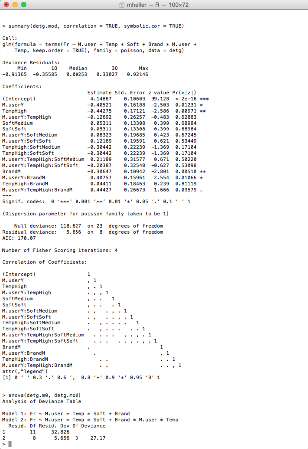
Figure 1. R running in a Bash shell, using the supplied glm.vr linear regression demo.

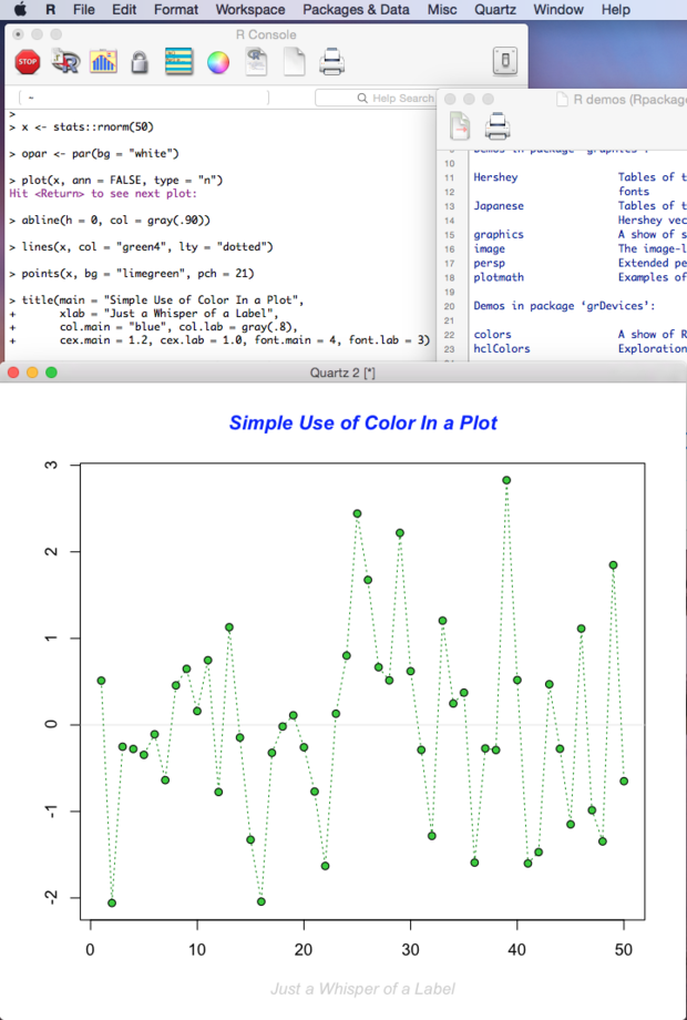
Figure 2. The R Console, a floating list of R demos, and a Quartz graphics window. The R graphics demo is running. Note that <- is the normal assignment operator.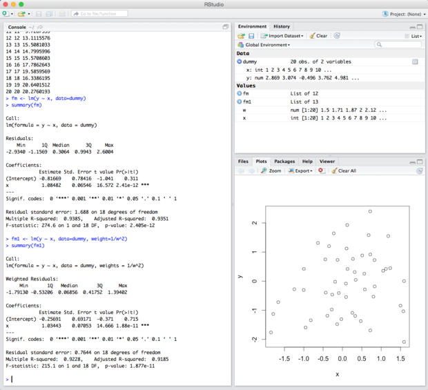

Figure 3. RStudio has four windows (all but the editor are shown here) and multiple tabs in each window. Sample code from the R site is running. Notice the data display in the upper right, which is quite convenient.

The power of R is illustrated by the deceptively simple calls in Figure 3 to do statistical analysis. For example,

fm1 <- lm(y ~ x, data=dummy, weight=1/w^2)
summary(fm1) 

This says “find the best fit coefficients, fitted values, and residuals for a linear model where y varies with x for the supplied data and weight vectors. Save them in object fm1 and then summarize the results.” Earlier in this session we had defined the following:

w <- 1 + sqrt(x) / 2

Reading this code is straightforward. Writing it takes a little study. But it isn’t hard and there’s lots of free help available, not to mention dozens of books.

In addition to the R help available on the Web and from the Help menu items in the R Console and RStudio, you can get help from the R command line. For example:

?functionName
help(functionName)
example(functionName)
args(functionName)
help.search("your search term")
??("my search term")

To get data into R, either use its sample data, listed by the data() function, or load it from a file:

mydata <- read.csv("filename.txt")

R is extremely extensible. The library() and require() functions load and attach add-on packages; require() is designed for use inside other functions. Many add-on packages and the R distributions live in CRAN, the worldwide Comprehensive R Archive Network. The other two common R archives are Omegahat and Bioconductor. Additional packages live in R-Forge.

The R installation copies the base packages and the recommended packages from CRAN into a local library directory, which on a Mac is currently at /Library/Frameworks/R.framework/Versions/3.1/Resources/library/. Running the R library() command without any arguments will list the local packages and the library location. RStudio will also generate the correct library() command to install a listed package when you check the installation check mark in the Packages tab. The command help(package = packageName) will display the functions in the specified package.

There are R packages and functions to load data from any reasonable source, not only CSV files. Beyond the obvious case of delimiters other than commas, which are handled using the read.table() function, you can copy and paste data tables, read Excel files, connect Excel to R, bring in SAS and SPSS data, and access databases, Salesforce, and RESTful interfaces. See, for example, the foreign package.

You don’t really need to learn the syntax for standard data imports, as the RStudio Tools|Import Dataset menu item will help you generate the correct commands interactively by looking at the data from a text file or URL and setting the correct conversion options in drop-down lists based on what you see.

You can see a list of the currently available packages by name on CRAN; this list is much more extensive than the list of recommended packages downloaded to your desktop by default. To install a package from one of the default archives, use the install.packages function:

install.packages("ggplot2")

Note that ggplot2 is a popular advanced graphics package that has more options than the standard graphics package. Nevertheless, graphics can do a lot. In addition to the graphics in Figures 2 and 3, consider Figures 4 and 5.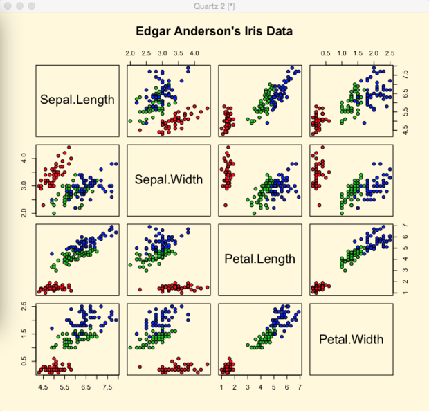

Figure 4. Edgar Anderson’s Iris data is a stock R data set, and this set of scatterplots was produced by the graphics demo.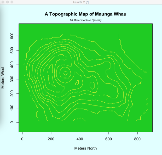

Figure 5. This topographic map of Maunga Whau was produced from stock data and thegraphics demo.

R can do much more in terms of graphics and statistical analysis. Do read Sharon Machlis’s tutorial and follow up with her links to additional information. At this point, I want to expand my discussion to how you can analyze big data in R.

R in the cloud

When R programmers talk about “big data,” they don’t necessarily mean data that goes through Hadoop. They generally use “big” to mean data that can’t be analyzed in memory.

The fact is you can easily get 16GB of RAM in a desktop or laptop computer. R running in 16GB of RAM can analyze millions of rows of data with no problem. Times have changed quite a bit since the days when a database table with a million rows was considered big.

One of the first steps many developers take when their program needs more RAM is to run it on a bigger machine. You can run R on a server; a common 4U Intel server can hold up to 2TB of RAM. Of course, hogging an entire 2TB server for one personal R instance might be a bit wasteful. So people run large cloud instances for as long as they need them, run VMs on their server hardware, or run the likes of RStudio Server on their server hardware.

RStudio Server comes in Free and Pro editions. Both have the same features for individual analysts, but the Pro version offers more in the way of scale: authorization and security, management visibility, performance tuning, support, and a commercial license. According to Roger Oberg of RStudio, the company’s intent is not to create paid-only features for individuals.

RStudio Server Pro is integrated with several big data systems. For example, when I was reviewing the IBM Bluemix PaaS, I noticed that R and RStudio are part of IBM's DashDB service (Figure 6). In fact, this is an installation of RStudio Server Pro on Bluemix and SoftLayer, according to Oberg and Tareef Kawaf of RStudio.

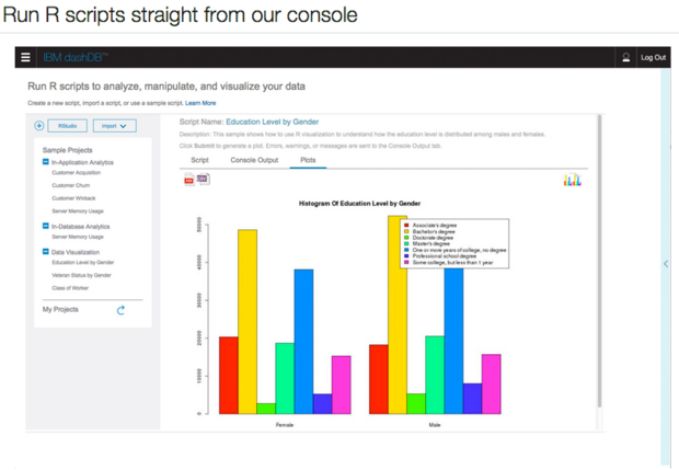
Figure 6. IBM Bluemix documentation touts the ability to run R scripts against a DashDB in-memory database.

There is an additional strategy for running R against big data: Bring down only the data that you need to analyze. In the spirit of MapReduce, Hadoop, Spark, and Storm, you want to winnow the data as you stream it to make in-memory analysis tractable on the reduced data set. To use Kawaf’s example, you may have 100TB of data but need “only” 5 columns and 20 million rows, a mere few hundred megabytes of reduced data.

You may also want to perform some of the analysis in the database instead of in the app. IBM has done a good job of providing an example, along with the R source code. Consider the analysis shown in Figure 7.

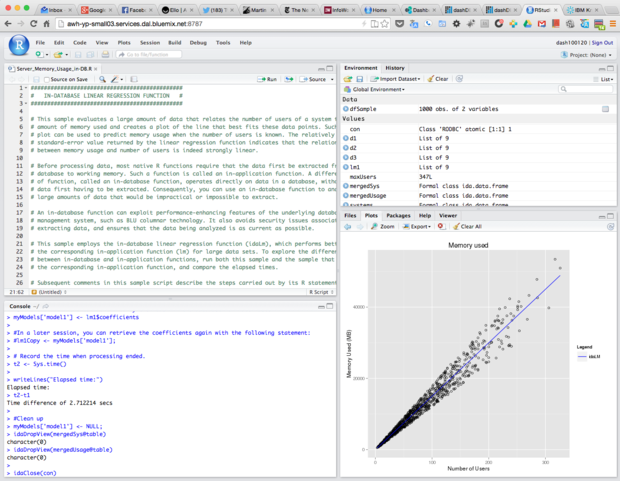
Figure 7. We are looking at RStudio Server Pro running in an IBM Bluemix dashDB service. The sample we ran did a regression from a large dataset in-database.

Streaming the data out of the database and into R can take a significant amount of time. If you eliminate most of the network streaming, you can vastly reduce the time needed for the analysis. You’ll notice that the timing for the in-database regression analysis is 2.7 seconds. The same task with the regression done in-application took 1.47 minutes -- more than 30 times longer. The regression coefficients computed were exactly the same. All that changed was that one analysis did the regression where the data resided, and the other first streamed the data from the database to the R application.

The IBM implementation is not unique; I happened to have a Bluemix account. Vertica (HP), Greenplum (Pivotal), Oracle, and Teradata all have R packages. I’m not sure how far the others have gone in the direction of in-database analytics, however.

By the way, I was pleasantly surprised to find that running RStudio Server Pro in a browser feels exactly like running RStudio on my desktop -- nicely done.

Shiny and R Markdown

Of course, developers and analysts never really get away with simply writing the code and determining the results. Top management wants monthly reports, and middle management wants to play with the data without knowing anything about what’s under the covers. Enter shiny and rmarkdown, two R packages from RStudio for Web applications and reporting, respectively.

Figure 8 shows a simple Shiny app running in RStudio. The code is from Lesson 2 of the Shiny tutorial.

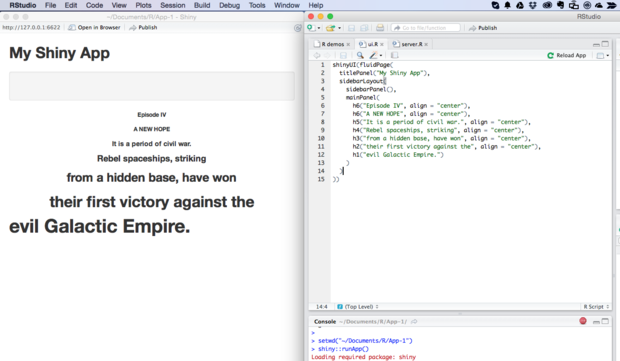
Figure 8. We’re seeing a Web page running a Shiny app, next to the RStudio editor showing the UI code for the app. The Shiny functions generate HTML. For example,h1("My title") generates <h1>My title</h1>.

You can use Shiny to build interactive and “reactive” Web apps, with widgets that correspond to HTML control elements such as input fields. By “reactive,” RStudio means that when a value changes, all values with dependencies on the changed value are recalculated, as you’d expect from a spreadsheet program. Figure 9 shows an interactive Shiny app with two widgets for input and a shaded choropleth map of U.S. census data for output.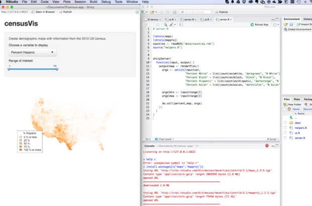

Figure 9. The U.S. map rendered in the example above changes when the user varies the input values. Note the readRDS base function to read a serialized R object, thesource function to include additional code, the renderPlot function (from the shinypackage) to render a reactive plot, and the do.call base function to construct and execute a function call. The percent_map function is defined in helpers.R to render the shaded county map and the state outline map.

The interactive Shiny app in Figure 9 is a good example of how you can allow middle management to play with the data without their having to know what’s under the covers.

To limit what is recomputed when input changes, the reactive wrapper function caches its values and recomputes only those that are invalid. I’ll forgo burdening you with an example, although you’ll find one in Shiny Lesson 6. Shiny apps can run on your own hardware, or you can publish them to the shinyapps.io server. For a quick example, have a look at Figure 10.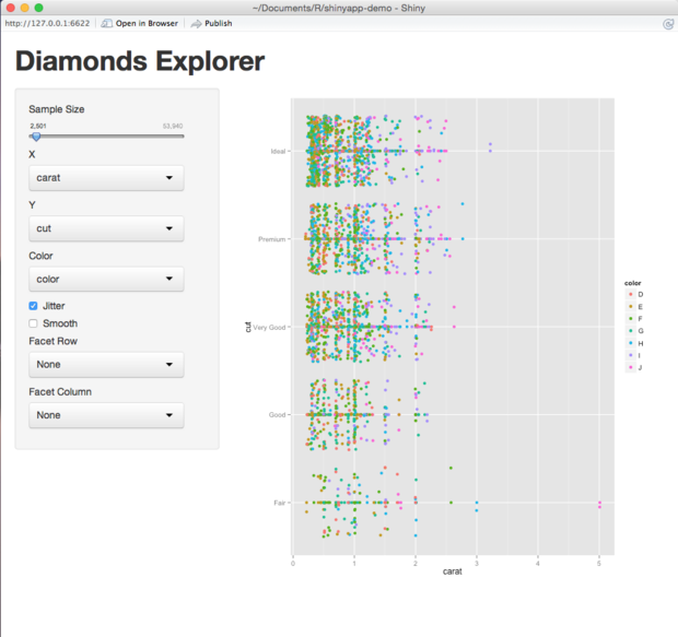

Figure 10. The interactive Shiny demo app running on my local system. You can run it yourself at https://mheller.shinyapps.io/shinyapp-demo/.

Shiny apps should satisfy the needs of middle managers. Now what about top management?

If you are a GitHub user or have simply been paying attention to the Web and developer landscapes the last 10 years, you’ll know about the Markdown language for generating formatted documents in HTML and other tag-based markup languages. RStudio includes a Markdown implementation and extends it to include embedded R code chunks and both LaTeX and MathML in the R Markdown package. You can also create interactive R Markdown documents using Shiny and publish them to your own Shiny server or to shinyapps.io. For an example, see Figure 11.

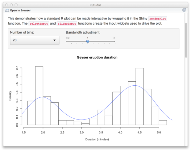
Figure 11. An example of R Markdown made interactive. The underlying code is a header block, a few lines of Markdown, and a dozen lines of R. See Figure 12.

Posted by Thiwanka Dilani